|
Using the method described above, length, girth and weight data from 67 fish [1] weighing 14.25 pounds or heavier were used to develop a new model based solely on the theoretical cylinder shown in Equation 5. The weight estimates from this model, deemed the 958 model for the value of the fit parameter, were then plotted versus the actual weights of the fish in study. Figure 1 shows the results of this exercise. An example of this model is shown below in Equation 6 with the 19.875 lb bass caught by Mike Long in 2004 which had Length and Girth measurements of 29.5 inches and 26.75 inches respectively.
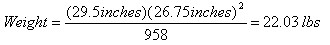 (6) (6)
Another method used in developing a weight estimation model was to keep the sum of the length and girth exponents equal to three but vary their values through a number of least squares curve fits. This would still give units of volume, which is dimensionally sound, but allows the modeler to not be constrained completely by the individual exponential values. An example can is shown in Equation 7.
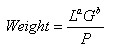 (7) (7)
where: a + b = 3
Starting out with the L exponent equal to zero and the G exponent equal to three, the exponential values were changed in increments of 0.1 until an L exponent value of three and G exponent value of zero was obtained. Then, by plotting the value of the L exponent versus the sum of the least squares analysis for each run, the optimum values for the L exponent and the G exponent were determined. An example of this model is presented below in Equation 8, again using Mike Long’s 19.875 lb bass[2].
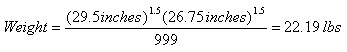 (8) (8)
The final method used for model development was a purely empirical method in which the exponents of length and girth are allowed to vary along with the fit parameter during a non-linear least squares regression. This method, although not theoretically based due to the fact that the sum of the exponents is allowed to deviate from units of volume, is commonly used when more theoretical methods do not produce satisfactory results. In essence, they are ways of estimating a desired outcome when some or all of the needed theoretical parameters (in this case density) are unknown. The outcome from this analysis provided the best “overall” results of the entire study except for fish over 20lbs where it underestimated the actual weight by up to 6%. Equation 9 gives an example of how this equation is used by again, using Mike Long’s bass. All of the above models and their results can be viewed in Figure 1 and Table 1.
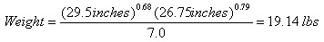 (9) (9)
Another method used to determine whether the models were more accurate for bass of a certain shape was a plot of the L/G Ratio versus the Weight Percent Difference in the model result with respect to the actual weight. Negative numbers show the model under-estimated the weight of the bass while positive numbers show a result that was over-estimated. A statistically sound model should always have an even number of results above and below the Zero Line. All of the models showed good distribution above and below the line but again, the empirically fit model produced the best results. See Figure 2.
Confidence intervals were also determined for each model in order to determine exactly how accurate each model was compared to actual weights. These intervals allow the user to determine not only the validity of the model but also the amount of error that can be expected for the interval chosen. For example, if a model has a confidence interval of +/- 4% at 90%, this means that 90% of the time, the model will be within 4% of the actual weight value. Three different intervals were determined, 90%, 95%, and 99%. The results of this analysis are shown in Table 2. The results show that again, the Empirical Model was by far the best in determining weight with the best certainty.
| 